Centroidal Model Predictive Control on a Quadruped
In this project, I implemented a centroidal MPC with Raibert heuristic swing leg controller to move a quadruped around in IsaacLab. This project was part of my core understanding for quadruped classical control, which is where my RL thesis stems from. By solving a QP, I was able to get the robot to follow a contact schedule and also a desired velocity.
Before the existence of more robust methods like Reinforcement Learning, MPC was the go-to option for controls scientists. It is fully based on math, and generates Ground Reaction Forces (GRFs) on the stance legs. In a quadruped robot, while moving, a gait will have some swing legs, and some stance legs. The swing legs will move to the next foot target in the direction of movement, while the stance legs will push against the ground and move the base of the robot to the desired position.
To achieve this strategy, one needs a method to calculate the swing leg foot target, and a method for stance leg forces. Overall, this method will deal in torque control, and is called Model Predictive Control (MPC). The swing leg method is called the Raibert Heuristic.

I run a diagonal leg trotting gait. Meaning on the quadruped robot, it will be front left and back right in swing while front right and back left are in stance, and vice versa. The swing legs foot targets are calculated using the raibert heuristic, the formula for which is shown to the right.
The heuristic is simple. When the robot is moving, it uses the swing leg time to calculate how far in front it needs to put the foot. If the robot is moving faster than desired, to slow it down, it will place the foot further in front of the robot, causing the base to decelerate. If the robot is going slower than desired, it will place the foot closer to the hip position, so the body accelerates. It was founded on the first hopping robot by Marc Raibert, so imagine this analogy on a pogo stick.

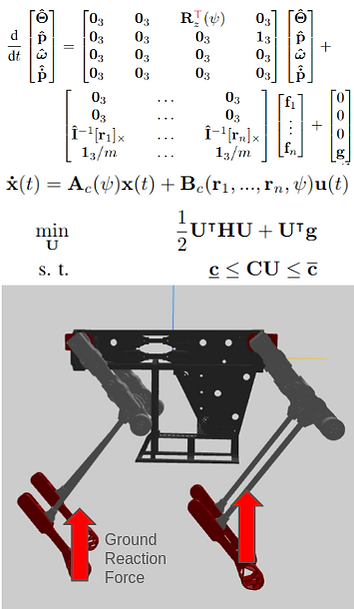
For the stance leg, the formulation of MPC is shown to the left. The first set of matrices are the dynamics of the translational and rotational components. So we want to find the change in state, which can be mapped using the rotation matrix of yaw Rz, moment arms from center of mass to the foot end I x r, and then a gravity state to compensate for the weight of gravity acting on the robot.
There are 13 states then: [euler angles xyz, position xyz, angular velocity xyz, linear velocity xyz]. So the formulation for the next state is given in a simple form of Ax + Bu. x is the state matrix, and u is the force matrix. So the A matrix maps changes in state, and B matrix maps changes in foot forces applied. With this, one can write the QP formulation subject to friction and force constraints. Finding the control force that satisfies the equation is the Ground Reaction Force (GRF). With the GRF, one can map it to torques on the joints using a Jacobian.
Shown below are the results for GRF tracking, swing leg trajectory tracking, the state of the robot center of mass, and a video of different velocities being matched by the robot. You can see that the joints move along the swing trajectory using simple Inverse Kinematics, and the robot is able to keep its base level.
The most challenging part of this was the gain tuning. Since each state needs a weight for the optimizer to consider, and there are 13 states, it creates a lot of possible combinations of gains to use. Other than that, understanding the math and writing the code for it was another major challenge. A small bug somewhere could lead to suboptimal solutions or just infeasible solutions.


Overall, this project taught me all about Quadratic Programming (QP), how MPC formulation is written, and bringing math into code. It gave me a strong understanding of the basics of legged robot control, and how I can use that for RL control that I am doing for my thesis in my research lab.